Technical case study
Understanding Market Exposure: A CAPM-Based Stock Evaluation
A CAPM-focused analysis estimating stock beta and alpha against the S&P 500 and using those coefficients to explore expected return.
The problem
This project emerged from a natural curiosity sparked during my earlier stock market analysis, where I explored daily return patterns and volatility trends. That initial exploration raised deeper questions: How do individual stocks behave in relation to market-wide movements? Can risk be quantified and priced? These questions led me to explore Beta (market sensitivity), Alpha (excess returns), and the Capital Asset Pricing Model (CAPM)—a foundational framework in modern finance.
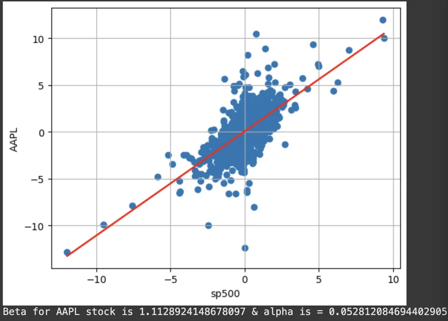
How sensitive is each stock to broad market movement, and how can that exposure be expressed through beta, alpha and CAPM expected return?
Approach
Rather than presenting the project as a notebook dump, this case study focuses on the decisions that shaped the analysis.
- Market benchmark analysis: Used S&P 500 as the market proxy and calculated average daily returns using .drop(‘Date’, axis=1).mean() to establish baseline market performance.
- Beta & Alpha computation: Applied np.polyfit() with order=1 to perform linear regression between individual stock returns and S&P 500 returns, extracting beta (slope) and alpha (intercept) coefficients.
- Batch analysis automation: Developed loops to iterate through all stocks (excluding S&P 500 and Date columns) using conditional statements if i != ‘sp500’ and i != ‘Date’ to calculate beta and alpha for each stock systematically.
- Interactive dashboard creation: Built Plotly Express scatter plots with px.scatter() and added regression lines using fig.add_scatter() to create interactive CAPM analysis charts for each stock.
- Risk metrics storage: Used Python dictionaries beta = {} and alpha = {} to store calculated coefficients for each stock, enabling easy comparison and further analysis.
Key implementation decision
Treat the S&P 500 as the common benchmark and automate the same regression across stocks
The same market-return series is used on the x-axis for every stock. Excluding the benchmark itself from the loop prevents a trivial self-regression from contaminating the comparison.
beta, alpha = np.polyfit(
    stocks_daily_return["sp500"],
    stocks_daily_return["AAPL"],
    1
)

rm = stocks_daily_return["sp500"].mean() * 252
rf = 0
expected_return = rf + beta * (rm - rf)Results & evidence
The figures below are the project evidence I would show first. The full implementation remains available through the GitHub link at the top of the page.
What challenged me
I initially struggled with the loop logic for batch processing all stocks because I was accidentally including the S&P 500 index in the analysis against itself, which created perfect correlation (beta = 1, alpha = 0) and distorted my results. After debugging, I realized I needed to exclude both ‘sp500’ and ‘Date’ columns using compound conditional statements if i != ‘sp500’ and i != ‘Date’ . This solution ensured I only analyzed actual stocks against the market benchmark, providing meaningful beta and alpha calculations for investment decision-making.
What I learned
- Beta turns visual market co-movement into an explicit sensitivity estimate.
- Automating the same regression across stocks makes comparisons consistent, but the benchmark itself must be excluded from self-regression.
- CAPM output depends on assumptions such as the benchmark and risk-free rate, so those choices belong in the interpretation.
What I would improve next
- Use a defensible contemporaneous risk-free rate instead of fixing it to zero.
- Add confidence intervals and goodness-of-fit measures around beta estimates.
- Test whether beta is stable through time using rolling regressions.
This project grew naturally out of the earlier stock-return exploration: once market-wide co-movement was visible, beta and alpha provided a way to quantify that relationship rather than only describe it visually.