Stock Price Analysis using Ridge Regression

The problem

This project focused on predicting future stock prices using historical data and Ridge Regression, comparing its performance to other models. I used Python and integrated both traditional machine learning and visualisation libraries to explore the data and build predictive models. Achieved an R-squared score of 98%, with a k-fold cross-validation score of 86%.

Approach

Rather than presenting the project as a notebook dump, this case study focuses on the decisions that shaped the analysis.

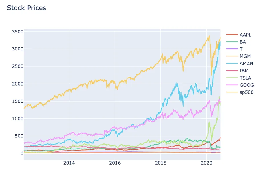
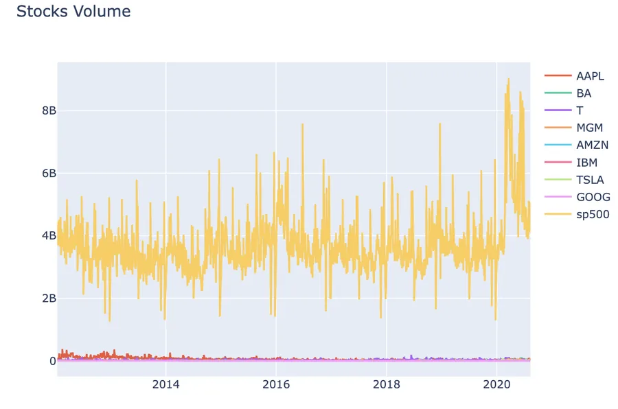
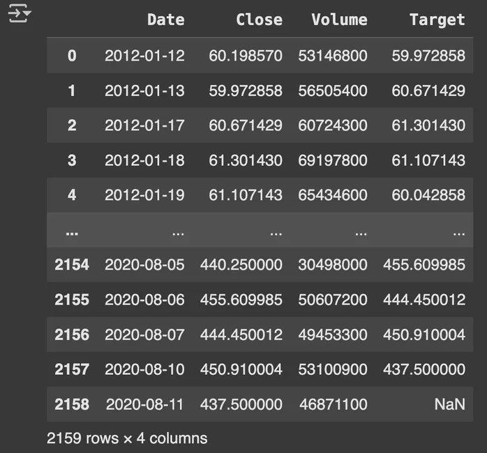
1. Load & inspect data: Loaded historical stock price and volume data from CSV files. Visualised trends in stock prices and volumes using line and distribution plots.
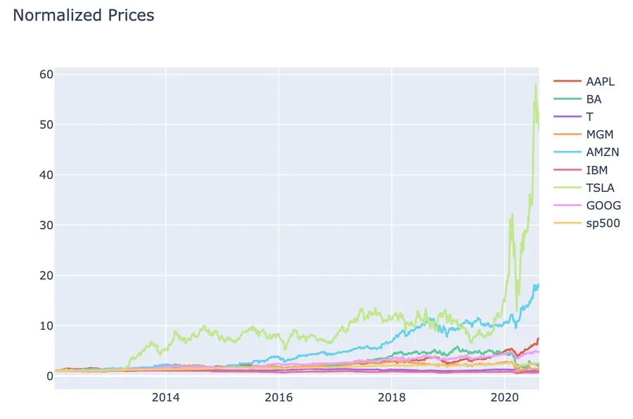
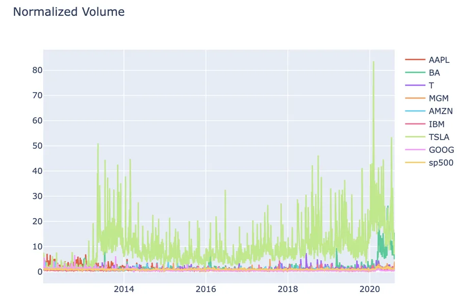
2. Preprocessing: Cleaned and aligned datasets by timestamps. Normalised features and created lag-based features for time series modelling.
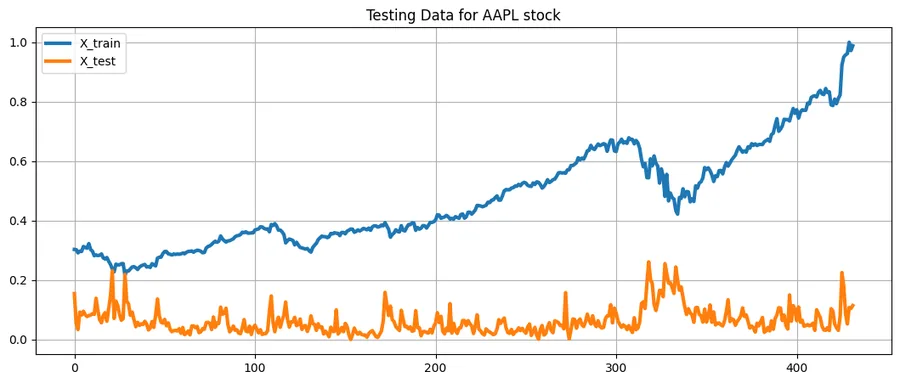
3. Model Development: Applied Ridge Regression to reduce overfitting from correlated features. Split dataset into training and testing sets using train_test_split().
4. Performance comparison: Evaluated models using r2_score .
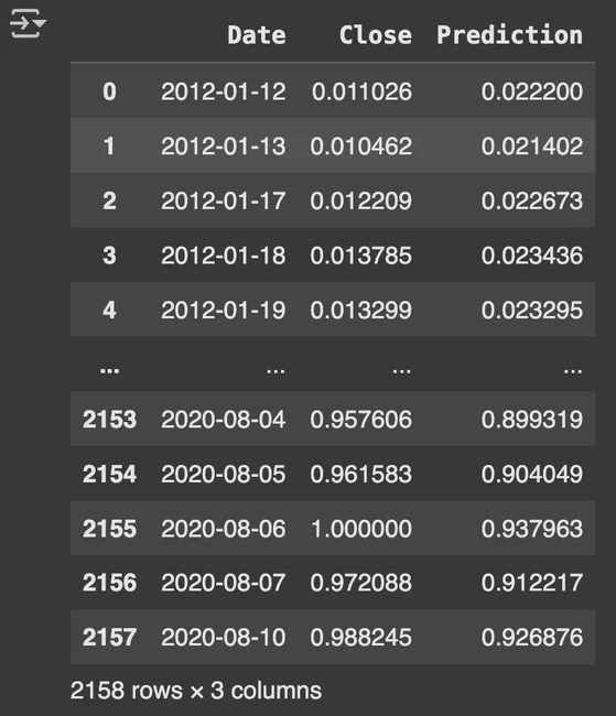
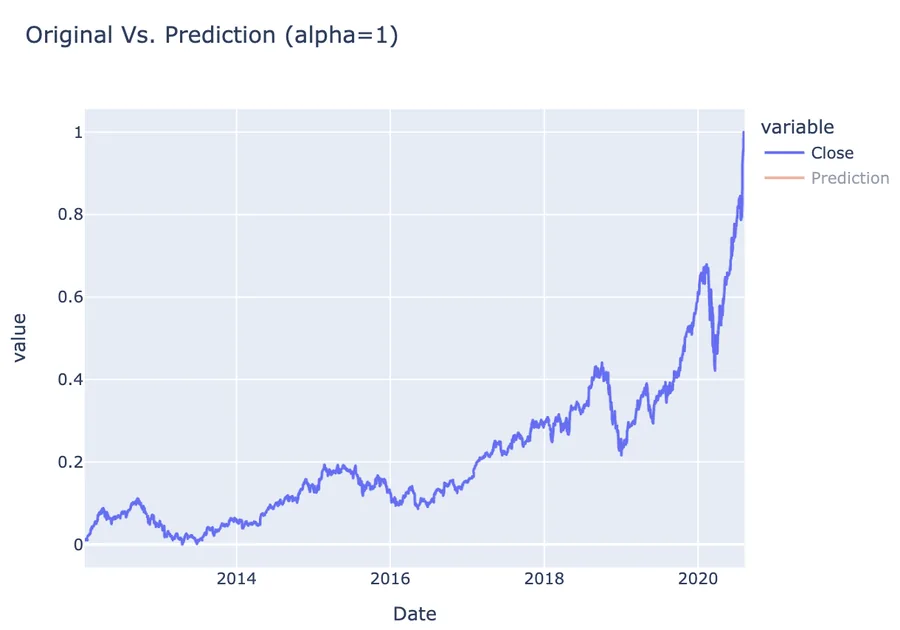
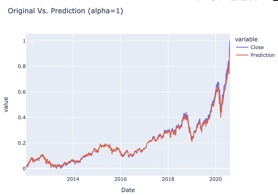
5. Visualisation: Plotted predicted vs actual stock prices to interpret model behaviour.

Key implementation decision

Use regularisation to control correlated financial features

Ridge keeps the linear modelling structure but penalises large coefficients. That makes it a useful baseline when price, volume and lag-derived features may carry overlapping information.

regression_model = Ridge()
regression_model.fit(X_train, y_train)

ridge_score = regression_model.score(X_test, y_test)
predicted_prices = regression_model.predict(X_test)

accuracies = cross_val_score(
    estimator=regression_model,
    X=X_train,
    y=y_train,
    cv=10
)

Results & evidence

The figures below are the project evidence I would show first. The full implementation remains available through the GitHub link at the top of the page.

What challenged me

Feature engineering for time series prediction was a significant challenge. Initially, using raw historical prices didn’t yield strong predictive accuracy. After adding lagged variables and scaling features, the model performance improved. It required careful experimentation to balance information richness and model simplicity.

What I learned

• Ridge is a useful linear baseline when predictors are correlated because L2 regularisation stabilises coefficient estimates.
• A strong in-sample or single-split score should not be interpreted as proof of robust forecasting performance.
• Time-series evaluation should preserve chronology instead of treating observations as exchangeable.

What I would improve next

• Use time-aware validation rather than ordinary K-fold splits for sequential data.
• Compare against persistence and unregularised linear baselines on exactly the same horizon.
• Report MAE/RMSE alongside R² and inspect residuals over time.