Technical case study
Stock Price Analysis using Long Short Term Memory Neural Network
A Tesla next-day price forecasting experiment using scaled price/volume inputs and a stacked LSTM network.
The problem
This project focused on predicting Tesla (TSLA) stock prices using deep learning techniques with LSTM neural networks. I built a time series forecasting model that uses historical closing prices and trading volumes to predict next-day stock prices, implementing robust validation through K-fold cross-validation.
Can an LSTM use recent Tesla price and volume information to model next-day closing-price behaviour?
The original experiment includes K-fold validation. For financial time series, I would now prefer walk-forward or expanding-window validation because chronology should be preserved during evaluation.
Approach
Rather than presenting the project as a notebook dump, this case study focuses on the decisions that shaped the analysis.
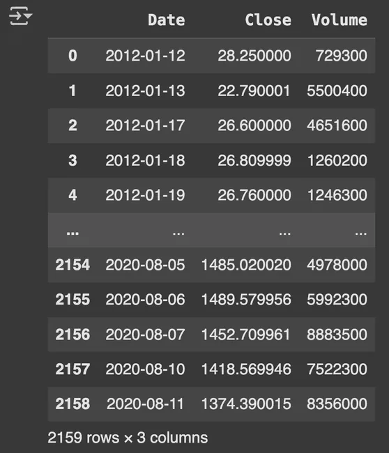
- Data Preparation: Combined separate stock price and volume datasets using custom individual_stock() function. Created target variable using trading_window() function with 1-day prediction horizon. Focused on Tesla (TSLA) stock as the primary case study.
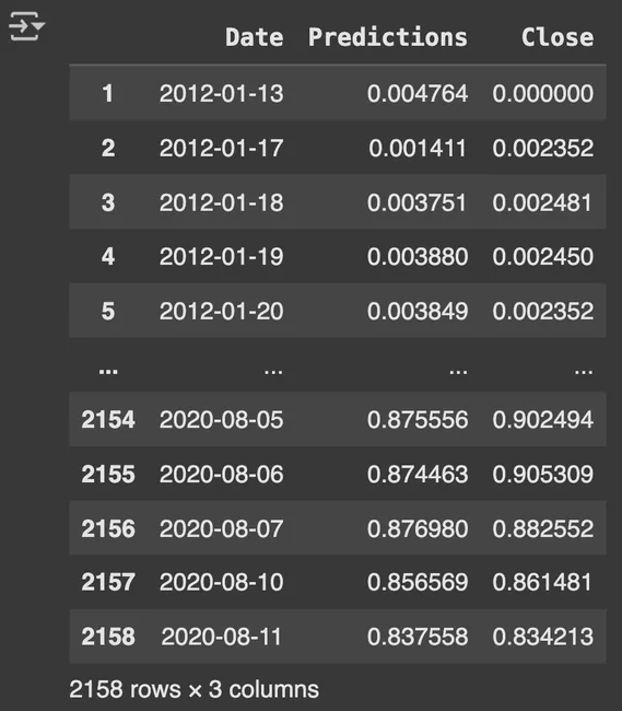
- Feature Engineering & Preprocessing: Applied MinMaxScaler to normalize closing prices and volumes to (0,1) range. Converted 1D arrays to 3D format required for LSTM input (samples, timesteps, features). Split data with 75% for training and 25% for testing.
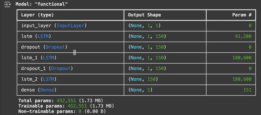
- Model Architecture: Built multi-layer LSTM model with three LSTM layers (150 units each). Implemented dropout layers (0.3 rate) between LSTM layers to prevent overfitting, used linear activation for final dense layer to output continuous price predictions and compiled with Adam optimizer and MSE loss function.
- Model Validation: Implemented 5-fold cross-validation to ensure model robustness, trained for 20 epochs with batch size of 32 and used 20% validation split during training for monitoring.
Key implementation decision
Reshape the time series explicitly into the tensor shape expected by the LSTM
The network expects data shaped as samples × timesteps × features. Making that transformation explicit prevents a silent mismatch between tabular arrays and sequence-model inputs.
sc = MinMaxScaler(feature_range=(0, 1))
training_set_scaled = sc.fit_transform(training_data)

X_train = np.reshape(
    X_train, (X_train.shape[0], X_train.shape[1], 1)
)

inputs = keras.layers.Input(shape=(X_train.shape[1], X_train.shape[2]))
x = keras.layers.LSTM(150, return_sequences=True)(inputs)
x = keras.layers.Dropout(0.3)(x)
x = keras.layers.LSTM(150)(x)
outputs = keras.layers.Dense(1, activation="linear")(x)Results & evidence
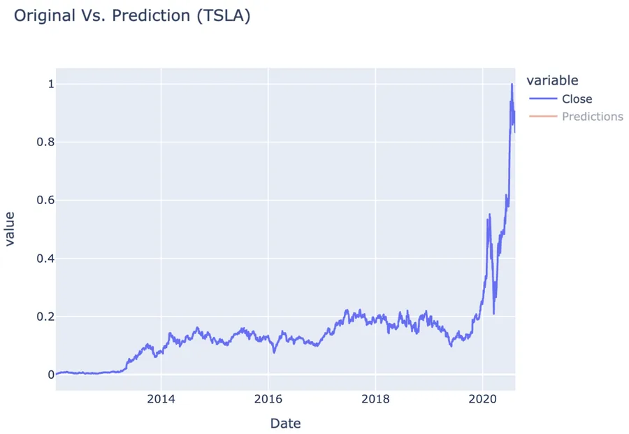
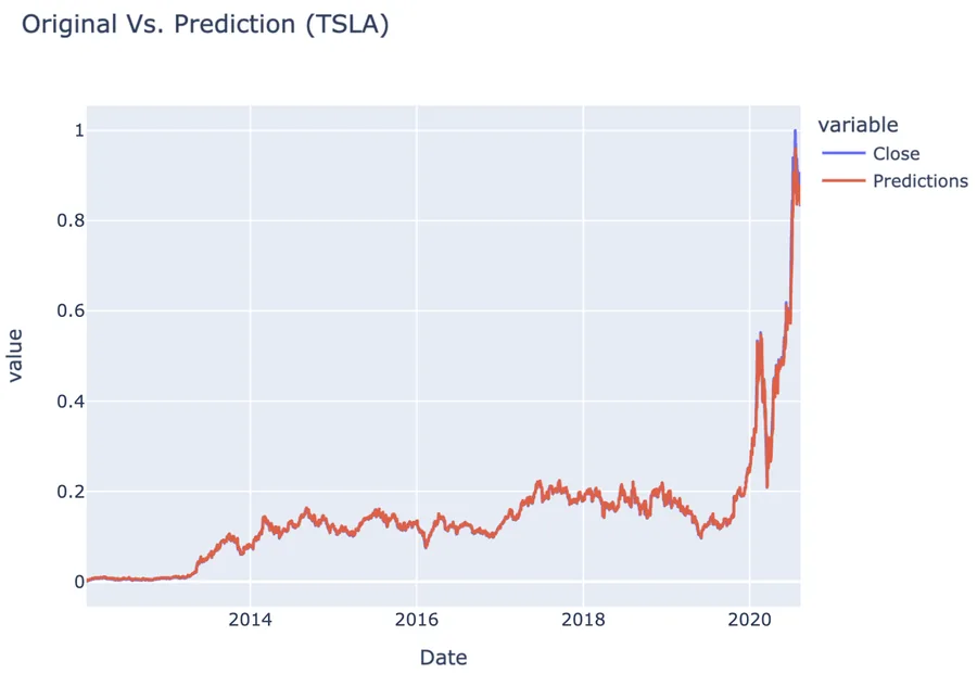
The figures below are the project evidence I would show first. The full implementation remains available through the GitHub link at the top of the page.
What challenged me
My biggest challenge was preparing the time series data in the correct 3D format for LSTM input. Initially, I struggled with reshaping arrays from 1D to the required (samples, timesteps, features) structure. After researching LSTM input requirements and experimenting with NumPy reshape operations, I learned to properly sequence the data with sliding windows and convert to the appropriate tensor dimensions for neural network training.
What I learned
- Sequence models require deliberate tensor shaping; tabular arrays cannot simply be passed into an LSTM unchanged.
- Dropout and stacked recurrent layers add modelling capacity, but evaluation design is at least as important as architecture complexity.
- Financial forecasting needs time-aware validation because random resampling can leak temporal structure.
What I would improve next
- Replace shuffled K-fold validation with walk-forward or expanding-window evaluation.
- Compare the LSTM against simple persistence and linear baselines.
- Use longer input windows and evaluate whether volume adds value beyond closing-price history.
This project is useful as a sequence-modelling exercise because it makes the data-shape requirements and architecture choices visible. The predictive result should still be interpreted cautiously because financial time series are non-stationary and evaluation design matters heavily.