Technical case study
HR Salary Prediction: Model Comparison
A small-regression comparison exploring how linear, polynomial, SVR, tree and ensemble models represent non-linear salary progression by position level.
The problem
This project compares regression approaches on a small position-level salary dataset. Because the dataset is tiny, I treat the exercise as a way to inspect model shape and preprocessing behaviour rather than as evidence of deployable salary prediction.
How do different regression families behave when the relationship between position level and salary is strongly non-linear?
Approach
Rather than presenting the project as a notebook dump, this case study focuses on the decisions that shaped the analysis.
- Data Preparation: Loaded position-salary dataset using pd.read_csv() and extracted features using iloc[:, 1:-1] (position levels) and target variable using iloc[:, -1] (salaries), strategically excluding the first column containing position titles.
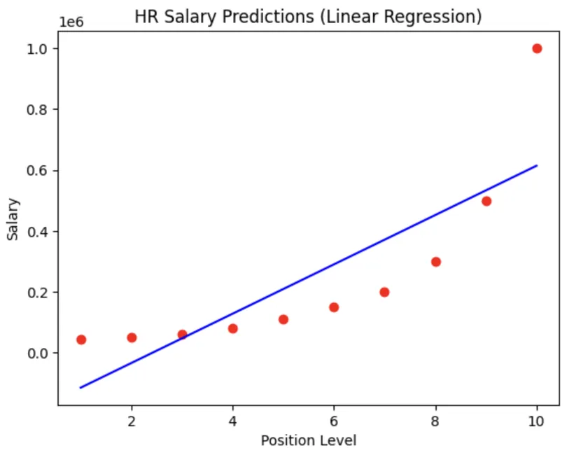
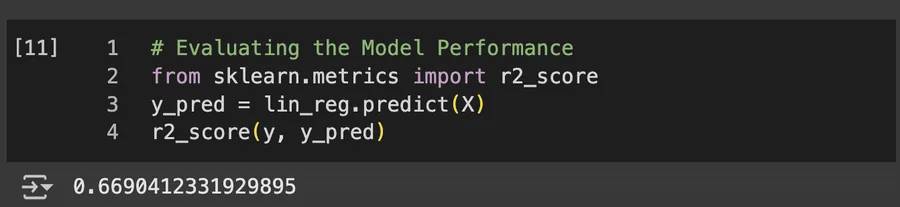
- Linear regression baseline: Implemented a standard LinearRegression() model using .fit(X, y) to establish a baseline for salary prediction based on position level with a straight-line relationship.
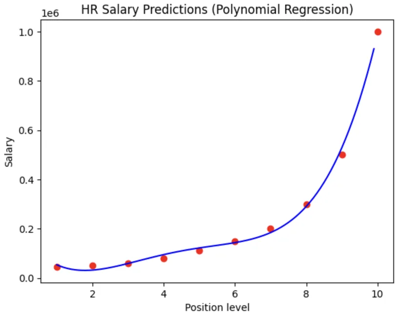
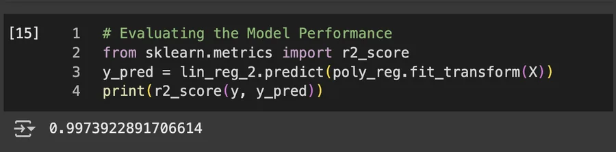
- Polynomial feature engineering: Applied PolynomialFeatures(degree=4) to transform the single position level feature into polynomial terms (x, x², x³, x⁴), creating a richer feature space to capture non-linear salary progression patterns.
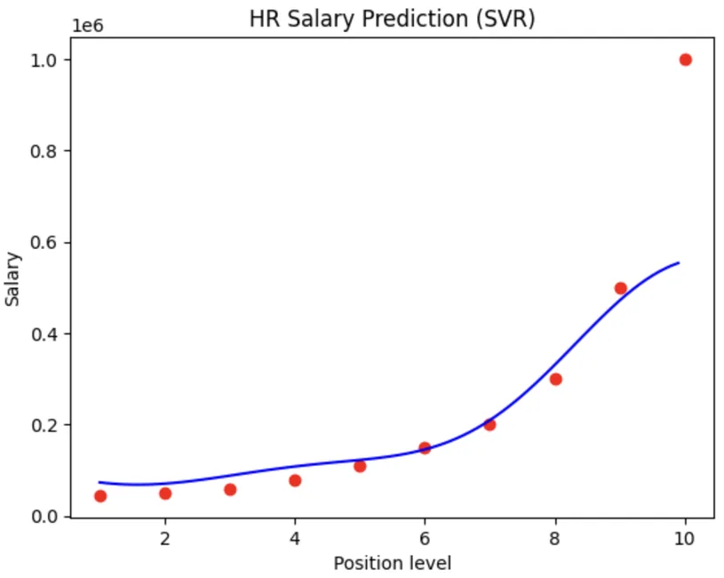
- Support Vector Regression: Implemented feature scaling using StandardScaler() for both X and y variables, then trained an SVR model with RBF kernel to handle non-linear relationships while managing the different scales between position levels and salary amounts.
- Decision Tree : Built a DecisionTreeRegressor() model that creates hierarchical decision rules to predict salaries, capturing complex non-linear patterns without requiring feature scaling.
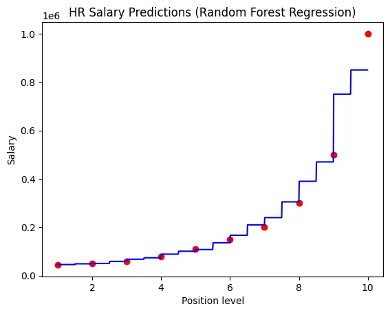
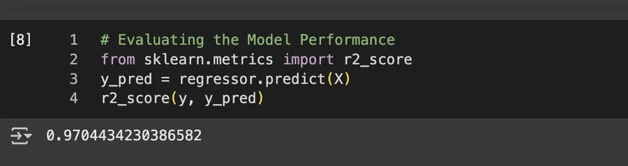
- Random Forest Regression: Implemented RandomForestRegressor() with multiple decision trees to reduce overfitting and improve prediction stability through ensemble learning.
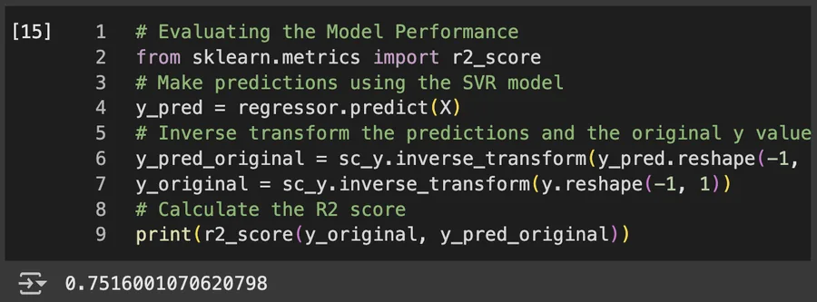
- SVR Inverse scaling: Applied sc_X.inverse_transform() and sc_y.inverse_transform() to convert scaled predictions back to original salary units, with proper reshaping using .reshape(-1, 1) for visualization.
Key implementation decision
Use dense prediction grids to make model shape visible
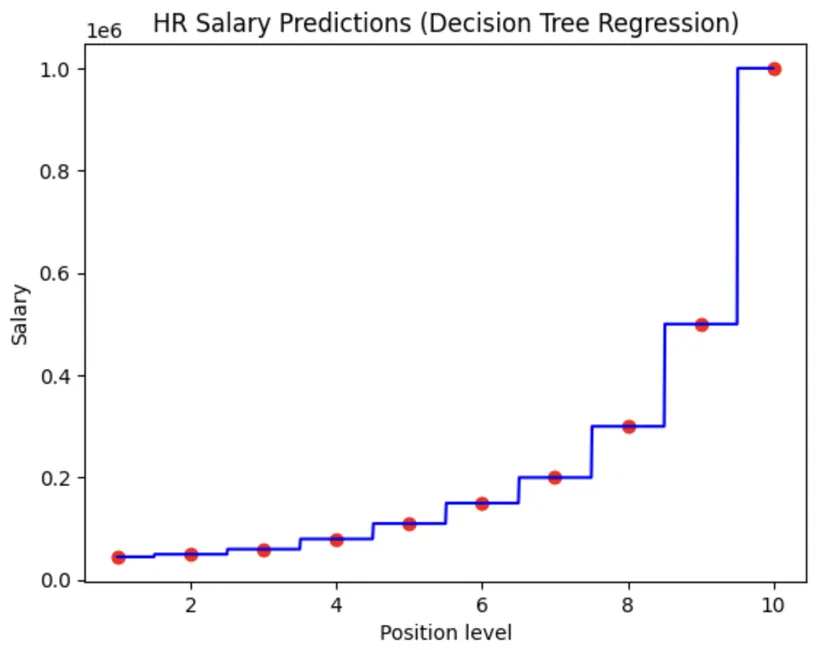
With a very small one-dimensional dataset, the plot is an important diagnostic. Increasing the grid resolution makes the stepwise behaviour of a tree model easier to see instead of implying a smooth relationship that the model does not learn.
regressor = DecisionTreeRegressor(random_state=0)
regressor.fit(X, y)

X_grid = np.arange(min(X), max(X), 0.01)
X_grid = X_grid.reshape((len(X_grid), 1))

plt.scatter(X, y, color="red")
plt.plot(X_grid, regressor.predict(X_grid), color="blue")Results & evidence
The figures below are the project evidence I would show first. The full implementation remains available through the GitHub link at the top of the page.
What challenged me
The SVR model visualization presented scaling complications because support vector regression requires feature scaling for optimal performance, but the visualization needed to display results in original salary units. The challenge was handling the forward and inverse transformations correctly. This was resolved by implementing a multi-step process: using sc_X.transform(X_grid) to scale the grid for SVR prediction, then applying sc_y.inverse_transform() to convert predictions back to actual salary values, with careful attention to array reshaping using .reshape(-1, 1) to maintain proper dimensionality throughout the scaling pipeline. This approach ensured accurate model performance while maintaining interpretable visualizations in original salary units.
What I learned
- Different regressors encode very different assumptions about smoothness and local behaviour.
- Dense prediction grids help reveal stepwise tree behaviour that can be hidden by sparse plotting.
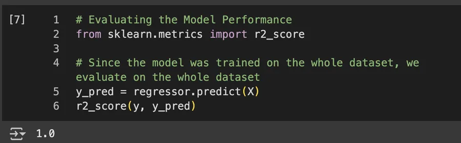
- With a very small dataset, visual fit is not evidence of generalisation.
What I would improve next
- Use a larger dataset before drawing conclusions about model generalisation.
- Introduce a proper holdout or resampling strategy once enough observations are available.
- Compare model complexity and extrapolation behaviour, not only fit on the observed points.
The dataset is deliberately small, so this page is most useful as a visual model-behaviour comparison rather than as evidence of generalisable salary prediction.