Technical case study
FashionMNIST Image Classification
A FashionMNIST computer-vision experiment comparing CNN architectures, with a TinyVGG-inspired model and detailed error inspection.
The problem
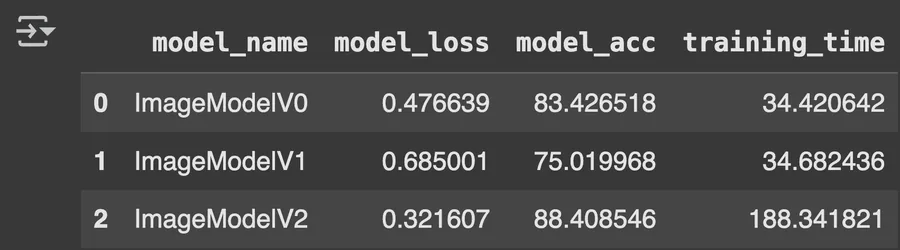
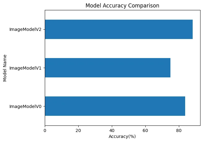
This project explores image classification using the FashionMNIST dataset, focusing on comparing CNN architectures to improve accuracy and training efficiency. It began as a practical extension of previous work in computer vision, driven by curiosity to deepen my understanding of how convolutional layers and activation functions impact learning. I designed a CNN inspired by the TinyVGG architecture and benchmarked it against two other models on performance and training time.
How much does a deeper convolutional architecture improve FashionMNIST classification, and where does it still confuse visually similar classes?
Approach
Rather than presenting the project as a notebook dump, this case study focuses on the decisions that shaped the analysis.
- Import & Setup: Loaded FashionMNIST using torchvision.datasets , transforming PIL images into PyTorch tensors.
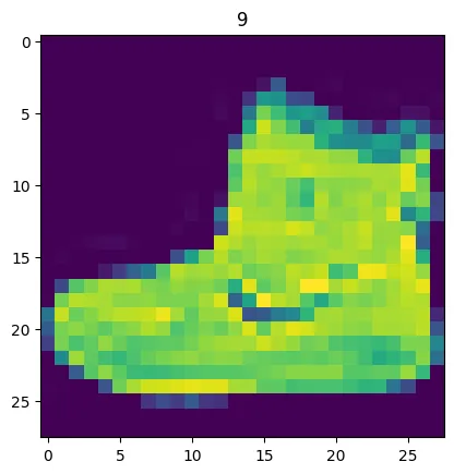
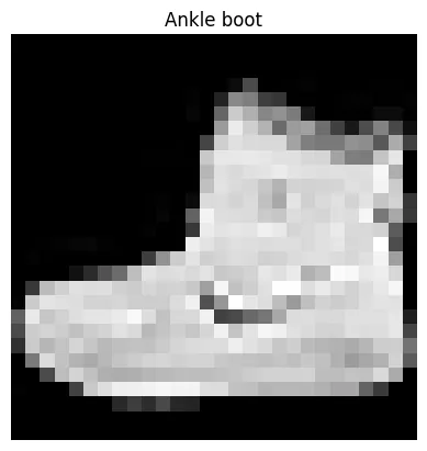
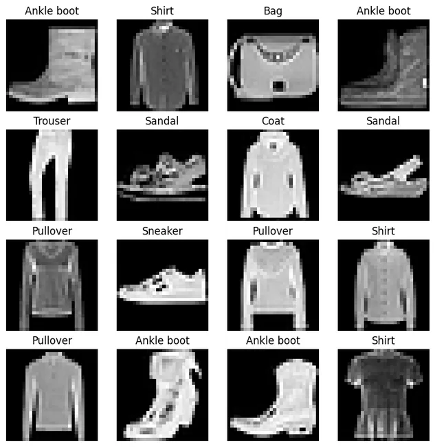
- Visual Exploration: Used matplotlib.pyplot to visualise images in grayscale and display class names, gaining familiarity with the data distribution (Figures A–C).
- Data Loaders: Implemented DataLoader objects with shuffling and batching (batch size = 32) for both training and test datasets.
- Model Definition: Constructed a CNN (TinyVGG-inspired) using nn.Sequential blocks for convolution, activation, and pooling, with a dynamically calculated flattened feature size for the final Linear layer.
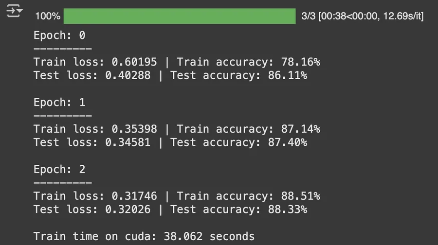
- Model Training: Trained the CNN using a loop with manual timing and CrossEntropyLoss . Tracked model accuracy with a custom accuracy_function .
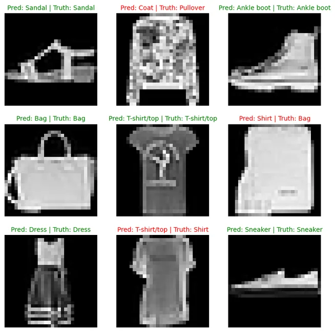
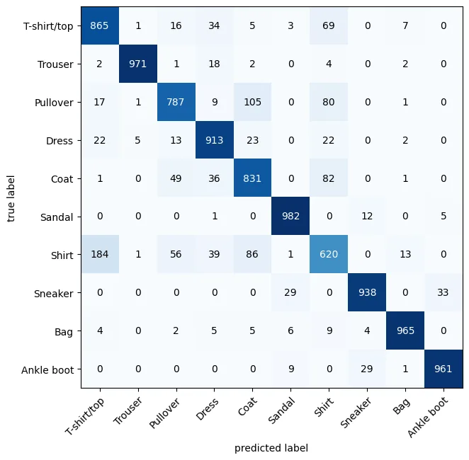
- Model Evaluation: Used a combination of random sample predictions, visual comparisons (Figure 3), and a confusion matrix (Figure 4) using TorchMetrics + MLXtend for deeper analysis.
Key implementation decision
Calculate the flattened feature size dynamically instead of hard-coding it
Convolution and pooling layers change spatial dimensions. Passing a dummy tensor through the feature extractor makes the classifier reusable and avoids manually recalculating the input size every time the convolutional blocks change.
with torch.no_grad():
    dummy_input = torch.randn(1, input_shape, 28, 28)
    x = self.conv_block_1(dummy_input)
    x = self.conv_block_2(x)
    self.flattened_size = x.view(1, -1).shape[1]

self.classifier = nn.Sequential(
    nn.Flatten(),
    nn.Linear(self.flattened_size, output_shape)
)Results & evidence
The figures below are the project evidence I would show first. The full implementation remains available through the GitHub link at the top of the page.
What challenged me
A key challenge was dynamically computing the flattened input size after the convolutional layers to correctly set up the first Linear layer. To solve this, I used a with torch.no_grad() block to pass dummy input through the conv layers and automatically extract the output shape. This approach prevented manual miscalculation and made the model reusable for different input sizes.
What I learned
- Deeper convolutional blocks captured spatial structure better than simpler baselines in this experiment.
- Error analysis exposed confusion between visually similar clothing classes that an aggregate score could hide.
- Computing the flattened feature size programmatically made the architecture easier to modify safely.
What I would improve next
- Test targeted augmentation for the classes that are most frequently confused.
- Use a validation set or cross-validation strategy consistently when comparing architectures.
- Profile training time and parameter count alongside accuracy so efficiency is part of the comparison.
The project was a practical way to connect convolutional architecture choices with model behaviour. The confusion matrix is especially useful because FashionMNIST contains categories that are visually similar even when overall accuracy is strong.