Technical case study
Customer Purchase Prediction – Model Comparison & Optimization
A classification comparison on social-network advertising data, using age and salary to predict purchase behaviour and visualise decision boundaries.
The problem
This project involved comparing multiple classification algorithms to predict whether users would purchase a product based on their age and estimated salary from social network advertisement data. I tested various models including Logistic Regression, SVM, Kernel SVM, Naive Bayes, K-NN, Random Forest, and Decision Tree. The Decision Tree classifier yielded the best results, which is why I’ve included its implementation in my portfolio.
Which classifier best captures the purchase boundary in a simple two-feature problem, and how does scaling affect both modelling and interpretation?
Approach
Rather than presenting the project as a notebook dump, this case study focuses on the decisions that shaped the analysis.
- Model Comparison & selection: Tested multiple classification algorithms (Logistic Regression, SVM, Kernel SVM, Naive Bayes, K-NN, Random Forest, and Decision Tree) to identify the best-performing model for this dataset.
- Data Import & Preparation: Loaded the Social Network Ads dataset using pandas and separated features (age, salary) from the target variable (purchase decision).
- Data Splitting: Used train_test_split() to divide the dataset into 75% training and 25% testing sets with a fixed random state for reproducibility.
- Feature scaling: Applied StandardScaler to normalize both age and salary features, ensuring equal contribution to the model since salary values are much larger than age values.
- Model Training: Implemented and trained seven different classifiers on the scaled training data: LogisticRegression , SVC (linear and RBF kernel) , GaussianNB , KNeighborsClassifier , RandomForestClassifier , and DecisionTreeClassifier with entropy criterion.
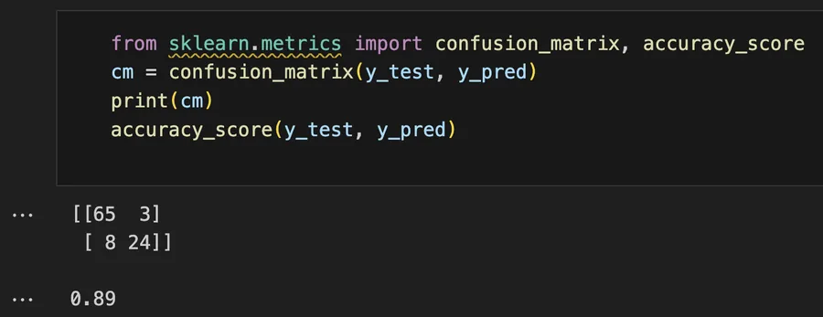
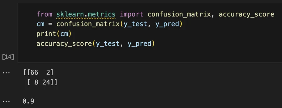
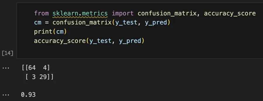
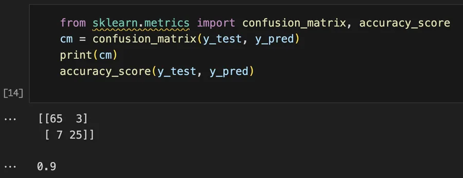
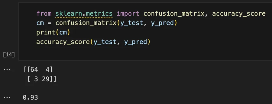
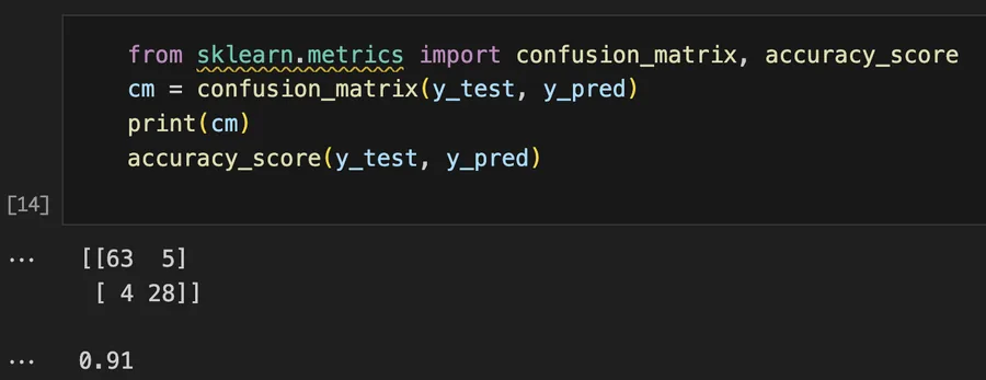
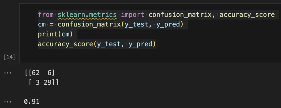
- Model Evaluation: Generated predictions on the test set and created a confusion matrix to assess classification performance and calculate accuracy score..
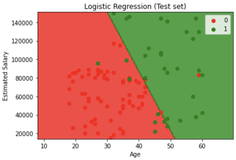
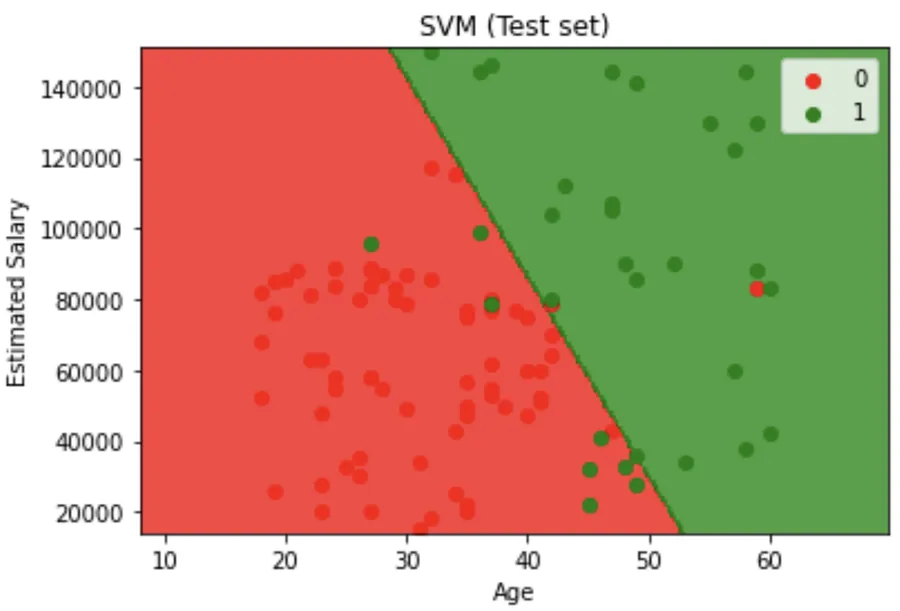
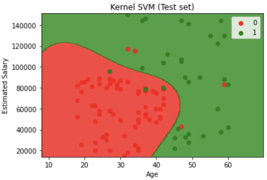
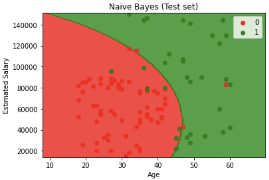
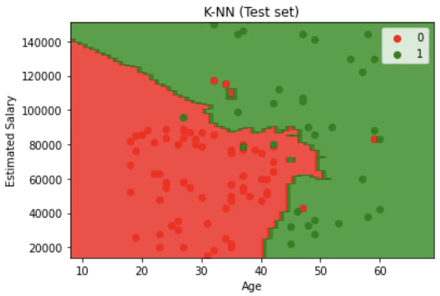
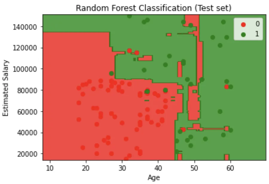
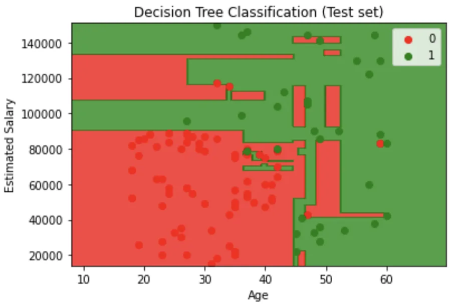
- Decision Boundary Visualization feature engineering: Created contour plots showing decision boundaries for both training and test sets, with red and green regions representing different classification zones.
Key implementation decision
Train in scaled space, explain in human-readable space
Scaling helps models treat age and salary comparably, but scaled coordinates make plots harder to interpret. The visualisation therefore inverse-transforms the features before displaying the learned boundary.
sc = StandardScaler()
X_train = sc.fit_transform(X_train)
X_test = sc.transform(X_test)

classifier = DecisionTreeClassifier(criterion="entropy", random_state=0)
classifier.fit(X_train, y_train)

y_pred = classifier.predict(X_test)
cm = confusion_matrix(y_test, y_pred)
accuracy = accuracy_score(y_test, y_pred)Results & evidence
The figures below are the project evidence I would show first. The full implementation remains available through the GitHub link at the top of the page.
What challenged me
At first, the visualisations were hard to understand because the data had been scaled. The age and salary values didn’t look realistic in the plots. I solved this by converting the data back to its original scale before plotting. This made the decision areas easier to read and relate to real-life values.
What I learned
- Feature scaling prevented salary magnitude from dominating age during model fitting.
- Inverse-transforming the features made the decision-boundary plots interpretable in real units again.
- A winning model on one split should be treated as a dataset-specific result until it is validated more robustly.
What I would improve next
- Compare models with cross-validation rather than a single holdout split.
- Report the full metric set instead of selecting the winner on accuracy alone.
- Use the two-dimensional setting to show where competing models disagree.
Because the dataset has only age and estimated salary as inputs, it is possible to inspect the classification surface directly. That makes the project useful for connecting model behaviour to a visual decision boundary.